LUPMIS

Annex 5: Possible Scenarios of GIS Analyses for ‘Land Use Planning’

The idea of this Annex is to give ideas to land use planners to derive and define analytical tools for GIS processing. Planners should define the relationship and conditions required for a new land use pattern, and then discuss it with the GIS modeling officer to enter it to LUPMIS. Listed examples are of textbooks, next version of this paper will have samples from Ghanaian data.

A5.1) Siting analysis:
Example here: Siting analysis of a wastewater treatment plant

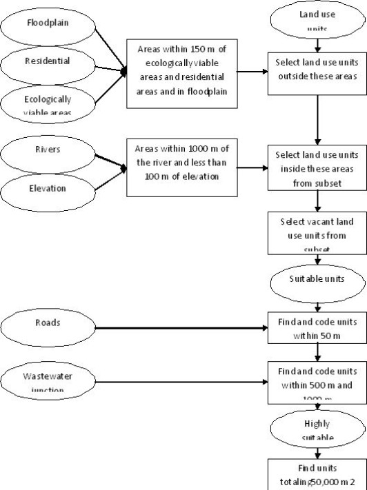
Figure A5.1: Siting analysis chart

This analysis consists of three phases.

In the first phase, you create a layer of the areas the plant should be outside of and another layer of the areas the plant should be within.

In phase two, you use these layers to select a subset of units that are in a suitable location. You then select the subset of these that are vacant to create a layer of suitable units.

In the third phase, you consider the town’s additional criteria that define the highly suitable units. You find the suitable units within 50 m of a road and those within 500 and 1000 m of the wastewater junction, then tag them with the appropriate codes so they can be identified on the map. You also check to see which units are large enough for the construction of the plant.

For this type of medium-complex analytical tools, it is important to have the entire process well documented.


A5.2) GIS analytical operations

• Union: Process to combine features in two input layers to create a new dataset;
• Intersect: Process as ‘Union’, but only area of overlap is preserved;
• Dissolve: Process to create a new layer in which all features in an input layer that have the same value for a specified attribute become a single feature;
• Merge: Process to combine any selected polygons, regardless of their attribute values;
• Split: Process to break a feature into two;
• Clip: Process of trimming feature in one layer using the boundaries of polygon features from another layer;
• Buffer: Process to create polygons of maximum distance around every feature in a layer, or at a distance that varies according to attribute values, representing a critical zone;
• Exclude: Process to eliminate areas;
• Calculate distances;
• Calculate areas;

create new map layers.

A5.3) 3D visualization

3-dimensional maps and figures help to visualize and to present spatial data, particularly to laymen. Amongst those, flooding demonstration is easy to compile and to demonstrate:

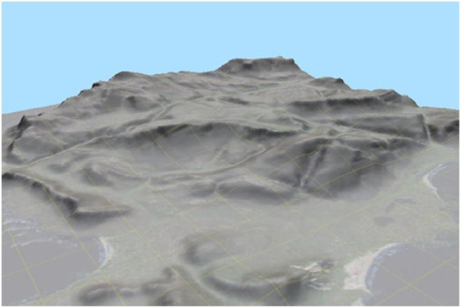
Figure A5.2: 3D visualization of terrain

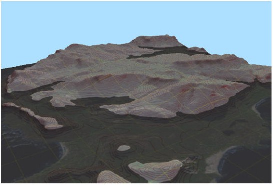
Figure A5.3: 3D visualization of terrain, with flood simulation

A5.4) Land use monitoring

GIS also performs as the appropriate tool for land use monitoring, i.e. the follow-up of land use plans and the recording, if land is being used in line with the land use plan, and that the plan is implemented.

The GIS is used to compare the land use plan, as approved earlier, with the actual land use.

• Phase 1: Current land use
• Phase 2: Land use plan (approved, in map form)
• Phase 3: After n years, newly assessed land use
• Phase 4: Comparison of map of phase 2 with map of phase 3, can be done utomatically, to result in identification of:

- Legal land use,
- Plan implementation areas,
- No change of land use,
- Illegal land use

Schematic, approved land use: Actual land use, after n years:

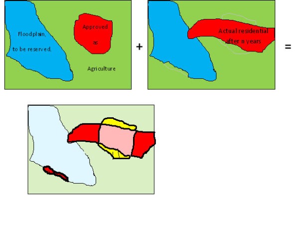
Orange: Residential, approved and implemented
Yellow: As residential approved, but not implemented
Red large units: Residential, but not approved as residential, illegal
Red small stripe: Illegally converted from flood reserve to agriculture

Figure A5.4: Land use monitoring sample

An actual sample map for land use monitoring looks like this:

Figure A5.5: Sample map of land use monitoring
(Bali, Indonesia, monitoring 1990-96, LREPP project)

• Colored areas show the new land use, where change took place
• White areas did not have a land use change

A5.5) Identification of areas under population forecast

Based on census data and area requirements of population, it is possible to forecast the need of space for future population, expressed in m2. This can be put on maps to visualize the spatial need for short, medium and long term planning of towns.

The same applies for the need of commercial, industrial areas and CBD.

A5.6) Density maps

Density maps take quantitative data of a DBMS and show their spatial density, for example of current or future population, of poverty (based on poverty indicators), of schools etc. Very often, they indicate a need for land use planning action.

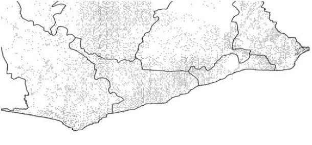
Figure A5.6: Community density in Southern Ghana

Copyright @ TCPD / LUPMP - version 2.0